Bauer

Here we will reproduce the results in the paper [1].

[1] : Carsten Bauer, Andreas Rückriegel, Anand Sharma, and Peter Kopietz. Non-perturbative renormalization group calculation of quasi-particle velocity and di-electric function of graphene. Phys. Rev. B, 92:121409, Sep 2015.

The exact FRG equations

\[\Lambda\partial_{\Lambda}v_{\Lambda}(k) = -\dfrac{e^2}{4\pi} \dfrac{\Lambda}{k} \int_{0}^{2\pi} d\phi \dfrac{ \cos(\phi)}{\epsilon_{\Lambda}\left(0,\sqrt{k^2 + \Lambda^2 - 2k\Lambda\cos(\phi)}\right)\sqrt{1-2(k/\Lambda)\cos(\phi) + (k/\Lambda)^2}} \\ = -\dfrac{e^2}{2\pi} \dfrac{\Lambda}{k} \int_{0}^{\pi} d\phi \dfrac{ \cos(\phi)}{\epsilon_{\Lambda}\left(0,\sqrt{k^2 + \Lambda^2 - 2k\Lambda\cos(\phi)}\right)\sqrt{1-2(k/\Lambda)\cos(\phi) + (k/\Lambda)^2}}\]

This equation can be turned into the usual form by substitution $\phi=2\varphi$.

\[\partial_{\Lambda}\epsilon_{\Lambda}(q) = \dfrac{2\pi e^2}{q} \partial_{\Lambda}\Pi_{\Lambda}(q) = -\dfrac{2e^2}{\pi}\int_{0}^{\frac{\pi}{2}}d\nu \dfrac{\theta(\frac{2\Lambda}{q}+\cos\nu-1)}{v_{\Lambda}(\Lambda)\Lambda + (\Lambda + q\cos(\nu))v_{\Lambda}(\Lambda+q\cos(\nu))} \\ \times \dfrac{q\sin^2(\nu)}{\sqrt{(2\Lambda + q \cos(\nu))^2 - q^2}}\]

The Code

Method 1

Using the method described in the usage

using FRGn

## Initialisation

const m = 304 # number of cutoffs
const n = 543 # number of momenta

velocity = zeros(n,m)
dielectric = zeros(n,m)

function velocity_integrand(velocity::Array{Float64,2},dielectric::Array{Float64,2}, momentum::Float64, cutoff::Float64, phi::Float64, m::Int64, n::Int64)
    ## Theta function implementation with conditional

    k = sqrt(cutoff^2 + momentum^2 - 2*cutoff*momentum*cos(2.0*phi))

    epsilon = get_dielectric(dielectric,k,cutoff,m,n)

    if k==0
        return 0.0
    else
        return 2.2*cos(2.0*phi)*cutoff/(pi*epsilon*momentum*k)
    end
end

function dielectric_integrand(velocity::Array{Float64,2},dielectric::Array{Float64,2}, momentum::Float64, cutoff::Float64, phi::Float64, m::Int64, n::Int64)
    ## Theta function implementation
    if cos(phi)<=1 - 2*cutoff/momentum
        return 0.0
    else
        k1 = cutoff
        k2 = cutoff + cos(phi)*momentum

        vel1, vel2 = get_velocity(velocity, k1, k2, cutoff, m, n)

        return 4.4*momentum*sin(phi)^2/(pi*(k1*vel1 + k2*vel2)*sqrt((k1+k2)^2 - momentum^2))
    end
end

## Boundary values initialisation
velocity[:,m] .= 1.0
dielectric[:,m] .= 1.0

## solving exact FRG using an user defined function from FRGn Package
rg_procedure(velocity,dielectric,velocity_integrand, dielectric_integrand ,m,n)

## Plots using user defined functions in FRGn Package
plot_velocity(velocity[:,1])

plot_dielectric(dielectric[:,1])

Method 2

There is also another method available in the package where at every cutoff an interpolated function (velocity and dielectric function as function of momentum) is used. The basic idea for using this method is exactly same as earlier.

NOTE: Same velocity_integrand and dielectric_integrand definitions will work here too.

using FRGn

## Initialisation
m = 123
n = 456

initial_velocity(momentum) = 1.0
initial_dielectric(momentum) = 1.0

velocity, dielectric = rg_procedure(initial_velocity, initial_dielectric, velocity_integrand, dielectric_integrand, m, n)

plot_velocity(velocity)
plot_dielectric(dielectric)

Both the methods internally uses the same methods but as this method uses interpolated function the result here is smoother(and more accurate) for smaller number of values of momentum (n).

Note that this method only returns the renormalised velocity and renormalised dielectric only compared to the previous method where velocity and dielectric function at all momentum and cutoffs were returned

Results

Renormalised Velocity	Renormalised Dielectric
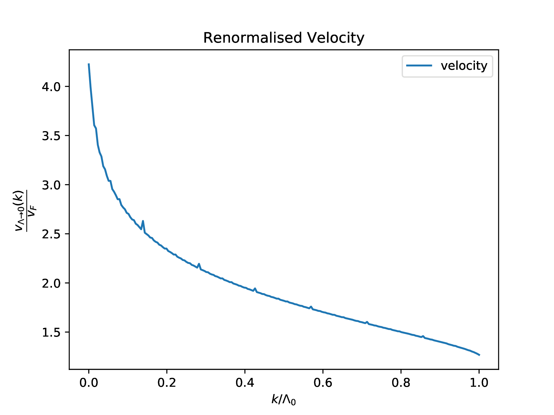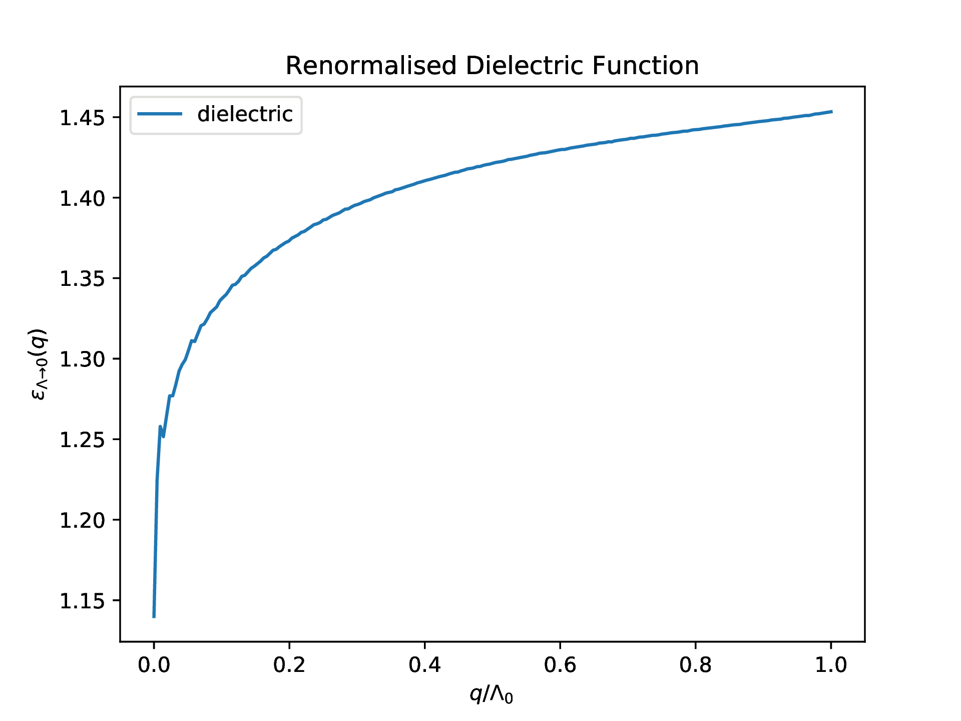